Jean-Baptiste Excoffier - Data scientist

Recent years have seen tremendous progress in automatic image analysis, either in classification, segmentation or compression task, as well as fictitious image generation (with GAN). This article focuses on image classification.

From examples where each image is associated to a certain class, Machine Learning models learn to identify patterns that are specific to a class so as to distinguish at best between the different groups.

The most efficient methods to date are based on neural networks, which are part of Deep Learning, that are now widely used in medical image research [1, 2]: early diagnosis of cancer cells, eye disease detection (AMD), or lung damage severity estimation of Covid patients.

We will present in this article characteristics of neural network models for image classification, through the evolution of their architectures.

Convolutions

Most machine learning models for classification work with tabular data. A list of several features, called explanatory variables, is passed to the model that will manipulate them (association, weighting)
in order to distinguish at best the different classes.

Yet an image is not a simple list of information in one dimension, but an object in two or three dimensions. The first and the second dimension respectively indicate image width and height while the third is added if there is need of colors, and not only greyscale image.

Thus in order to use this kind of classical classification model, image must be initially flattened to have a one-dimension object, consisting in a list of pixels.

Figure 1 shows this process with a four pixel image and a very simple neural network called Multilayer Perceptron. It is only made up of a single intermediate layer (FC for Fully Connected) of five neurons. After image flattening, each pixel is linked to all neurons.

Each connection is associated to a coefficient indicating the weight the model gives to it. It is these coefficients, also called parameters or weights, that the model will optimize duing its learning phase, by attributing the value that enables the best distinction between every classes.

The last layer (Exit) gives for each image the class predicted by the model, or the probability of belonging to each class.

Nevertheless, image flattening does not fully take into account the spatial distance between pixels, which is an obvious limit to model performances. Moreover, flattening produces a list -a vector- of a very large size. Our first example only consists in a 2×2 image, so the vector has a length of 2×2 = 4 pixels, but for an image with a normal size, such as 300 × 300, is thus generates a vector fo 90,000 pixels, which must be multiplied by 3 if it is a color image (RGB).

Therefore, we need a method that can extract information and patterns from spatial proximity and intensity of pixels in order to better take into account colors and forms.

Convolution filter, also called kernel or mask, is such a method that modifies an image based on a matrix, highlighting certain area or aspects. This convolution matrix, that must be smaller than the image, runs through the image, from left to right and from top to bottom, generating at each position a number that will be a pixel of the new image produced by the convolution operation.

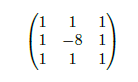
An example of convolution filter is given by matrix 2. It has a 3 × 3 dimension and is used for contour detection of objects contained in the image. It is also useful to be able to diminish the image size, in particular to have a fewer number of parameters in the model.

This is possible by modifying the stride of the convolution operation so as to skip a certain number of pixels while running through the image. If the stride is one then the generated image is of the same size than the original, but if the stride is equal to 2 than the generated image will be half the size of the original.

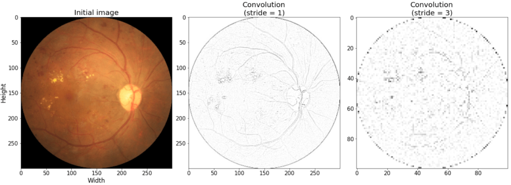
Let’s take an example of an ophthalmologic exam consisting of fundus image for the detection of diabetic retinopathy [3] from a open source dataset https://github.com/HzFu/EyeQ.

Figure 3 shows the original image of a patient suffering from diabetic retinopathy, and the result of the convolution operation from filter 2, with two different values of the stride parameters. With a stride of 1, the blood vessel contours are well detected, while a stride of 3 produces an more blurred image but smaller (axis indicate size).

Thus we have a technique that takes into account the spatial side of the imagery. Although it is not the only technique used in the current neural networks of image processing, there is in particular the pooling, the convolution remains the principal and especially the only one having coefficients (or weights, parameters), whose values the model will be able to choose according to the data.

For example, we could build a model with filter 3, but instead of choosing the coefficients a priori, the model would learn to optimize them in order to have the best possible accuracy for the classification. This filter would thus have 3 × 3 = 9 weights to optimize, to which a common weight must be added (as in a linear regression ax + b). For color images, number of weights must be multiplied by 3 (RGB channel), which for a convolutional kernel of size 3 × 3 gives a total of 3 × 3 × 3 + 1 = 28 parameters.

Convolution operations are detailed in the following article [4].

First architectures

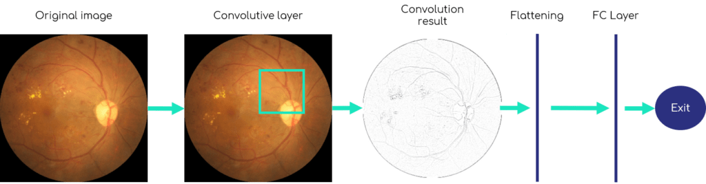
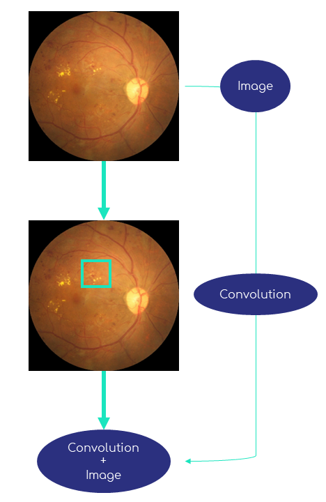
A very basic architecture of a neural network model containing convolution, also named Convolutional Neural Network (abbreviated in ConvNet or CNN), consists of a first layer with a convolution filter, then a flattening of this result followed by a completely connected layer (Fully Connected), and finally the output of the model which is often a vector of probabilities (one for each class, the whole summing up to 100%).

Figure 4 shows this basic architecture. Here the size of the convolution filter (the square with the yellow edges in the second image) is voluntarily enlarged, because in general this one is relatively small, from 1 × 1 to 5 × 5 pixels.

The first architecture of CNN is published in 1998 [5]. It is not much more complex than the figure 4, since it only consists of two convolutional layers followed by three completely connected layers. This model, named LeNet-5, has about 60,000 parameters and was applied to the recognition of digits in bank checks and postal codes.

Nevertheless, the low capacities of previous computers prevented a good training as well as the use of more complex and deeper models with more layers.

2012 was a real breakthrough in the complexity of convolutional networks, with the article [6] presenting the AlexNet model. Although not very different in substance from the LeNet-5, this new model is deeper and contains many more parameters, about 12 millions. In 2014, the model VGG-16 [7] saw a considerable increase in depth -13 convolutional layers versus 5 for AlexNet- thus in the number of parameters to optimize (138 million) [7].

Therefore, the models had become very heavy, mainly due to the new and great capacity of computers to be able to manage these enormous neural networks. From then on, the research will more and more focus on the improvement of architecture efficiency and not just a simple increase of parameter number.

Inception Architectures

A way of improving the performance of neural networks is to increase not only depth, but also the model width. While previously the convolutional layers were just following each other, the Inception-V1 model published in the article [8] in 2014 uses convolution filters put side by side in blocks called Inception.

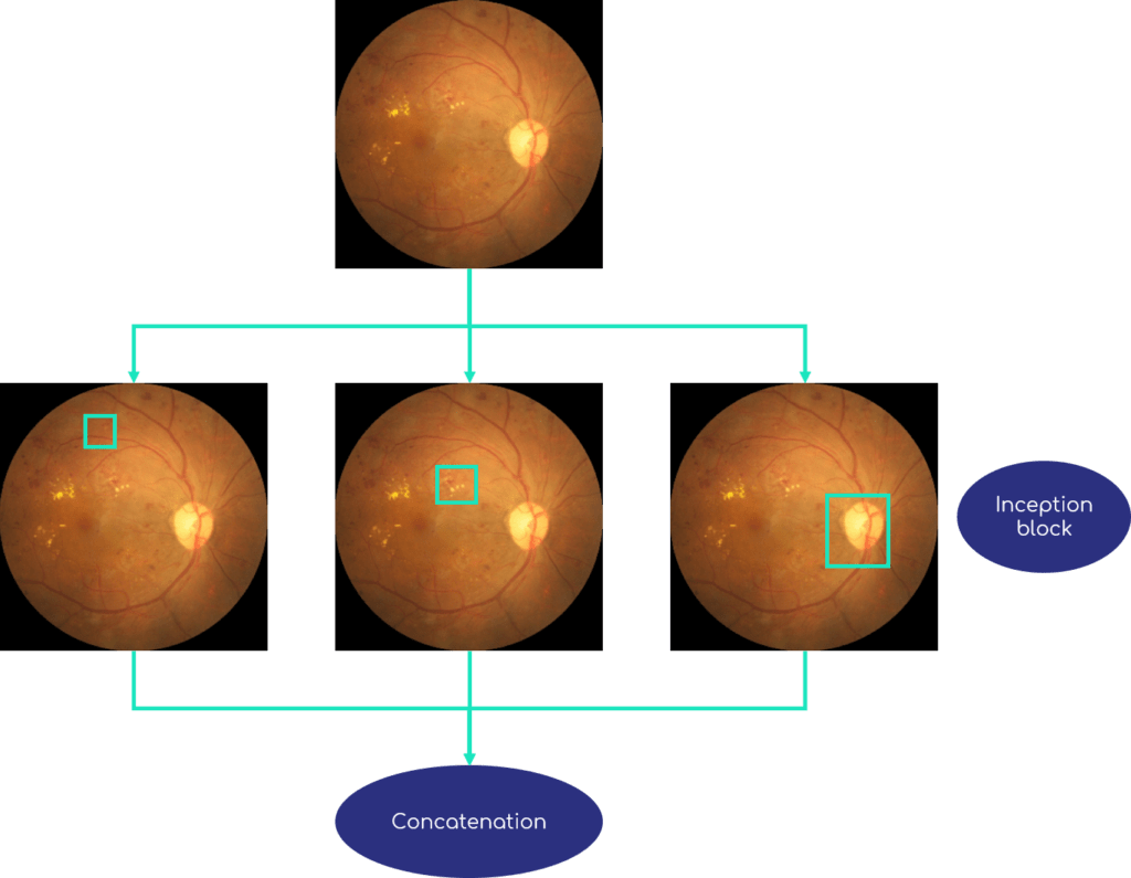
Each block contains several convolutions of different dimensions, in order to extract information of different sizes. The small convolution filters focus on small areas of the image, while larger filters capture more global information.

Figure 5 shows an example of an Inception block. The image or the previous layer, is processed in parallel by convolution filters of several sizes : blue, red and violet squares. Sizes are exaggerated here to make them visible, normally filter dimensions are often 7 × 7 pixels at maximum. Then the different information is concatenated to be passed in one piece to the next layer.

A significant improvement of Inception-V1 was released in 2015, named Inception-V3 [9]. The advances are mainly related to the factorization of convolution filters, by decomposing for example a filter n × n into two : the first one of dimension 1 × n followed by a filter of size n × 1.

The Inception architecture greatly improved model performances while lowering learning time, in particular by reducing number of trainable parameters : only 5 millions for Inception-V1 and 25 millions for Inception-V3, whereas VGG-16 contained 138 million neurons. Nevertheless, problems persisted during the learning process, problems that will be mostly corrected by future architectures.

Residual Architectures

A major problem in neural network training is the vanishing gradient problem. Training is iterative : at each step the parameter values (or weights, neurons) are adjusted in order to improve the model performance. To each initial value is added its gradient, which indicates the direction (positive or negative gradient) and the level of adjustment necessary to minimize an error function. But often this gradient can be equal to zero, preventing a real update of parameters. This can happen after a good number of iterations, which is normal and corresponds to the end of learning process since the network is no longer able to draw new relevant information from the images to improve itself. But the vanishing gradient could also occur very quickly, after a few steps, which is a problem since it comes from a numerical error.

Moreover, the common belief at the time was that increasing the depth of a model automatically improved its performance. However, this did not translate into practice since some less complex models managed to beat deeper models.

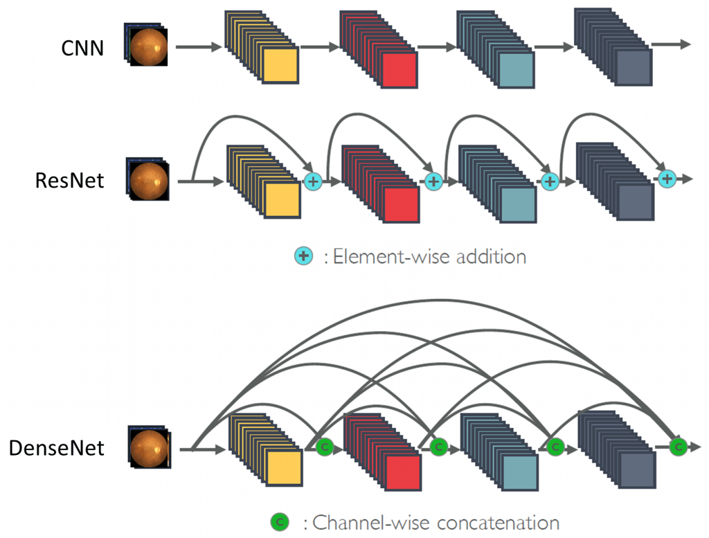
In 2015 are introduced the Residual networks, also called ResNet, in the article [10]. Their particularity is that at each block, the input is redistributed to the output, as shown in figure 6. Thus the model only learns the effects of convolution, without depending on the initial input, allowing a better generalization and efficiency, hence the term residual since learning is done on the difference between input and output (thus the residual) and not on pure output. Moreover, the vanishing gradient problem is very often avoided with this architecture.

Since then, several improvements to these residual networks have been made. An approach combining the Inception and Residual architectures is first proposed in 2016 [11] (Inception-ResNet), then in 2017 [12] (ResNeXt).

Another axis of improvement is brought by the so-called dense models (DenseNet), first published in 2017 [13]. This architecture does not use the Inception blocks, but pushes the concept of the ResNet to the maximum. While in the latter, only one link is added per convolutional block, a densely block transmits its input to all the following blocks, as shown in figure 7. This architecture is to date one of the most efficient, with the Inception-ResNet [14].

Conclusion

Automatic analysis of medical images, especially for classification purposes, has made significant progress in recent years. The increase in computational capacities as well as the improvement of Deep Learning methods, of which we have described the long evolutions ([15]) in this article, have allowed a significant increase in classification model accuracy, as much as to consider their use in a real clinical setting in order to assist practitioners, particularly for early detection of diseases.

Nevertheless, some problems concerning neural network models are regularly raised, such as their reliability and consistency. Indeed, a model, even if efficient, can be based on areas of the image considered to be of little or no clinical relevance by physicians. This can happen when the model is based on images containing artifacts that are more present in one class than another.

Consequently, it is essential to better understand how neural networks work and behave, especially for individual diagnosis by visualizing areas considered by the model as being the most important in its decision making.

Several techniques, grouped under the notion of explicability, have been developed in recent years. The next article describes the state of the art in this field, and its use in medical imaging.

Références

[1] G. Litjens, T. Kooi, B. E. Bejnordi, A. A. A. Setio, F. Ciompi, M. Ghafoorian, J. A. Van Der Laak, B. Van Ginneken, and C. I. Sánchez, “A survey on deep learning in medical image analysis,” Medical image analysis, vol. 42, pp. 60–88, 2017.
[2] S. K. Zhou, H. Greenspan, C. Davatzikos, J. S. Duncan, B. van Ginneken, A. Madabhushi, J. L. Prince, D. Rueckert, and R. M. Summers, “A review of deep learning in medical imaging : Imaging traits, technology trends, case studies with progress highlights, and future promises,” Proceedings of the IEEE, 2021.
[3] “Rétinopathie diabétique - snof.” https://www.snof.org/encyclopedie/r%C3% A9tinopathie-diab%C3%A9tique. Accessed : 2020.
[4] V. Dumoulin and F. Visin, “A guide to convolution arithmetic for deep learning,” arXiv preprint arXiv :1603.07285, 2016.
[5] Y. LeCun, L. Bottou, Y. Bengio, and P. Haffner, “Gradient-based learning applied to document recognition,” Proceedings of the IEEE, vol. 86, no. 11, pp. 2278–2324, 1998.
[6] A. Krizhevsky, I. Sutskever, and G. E. Hinton, “Imagenet classification with deep convolutional neural networks,” Advances in neural information processing systems, vol. 25, pp. 1097–1105, 2012.
[7] K. Simonyan and A. Zisserman, “Very deep convolutional networks for large-scale image recognition,” arXiv preprint arXiv :1409.1556, 2014.
[8] C. Szegedy, W. Liu, Y. Jia, P. Sermanet, S. Reed, D. Anguelov, D. Erhan, V. Vanhoucke, and A. Rabinovich, “Going deeper with convolutions,” in Proceedings of the IEEE conference on computer vision and pattern recognition, pp. 1–9, 2015.
[9] C. Szegedy, V. Vanhoucke, S. Ioffe, J. Shlens, and Z. Wojna, “Rethinking the inception architecture for computer vision,” in Proceedings of the IEEE conference on computer vision and pattern
recognition, pp. 2818–2826, 2016.
[10] K. He, X. Zhang, S. Ren, and J. Sun, “Deep residual learning for image recognition,” in Proceedings of the IEEE conference on computer vision and pattern recognition, pp. 770–778, 2016.
[11] C. Szegedy, S. Ioffe, V. Vanhoucke, and A. Alemi, “Inception-v4, inception-resnet and the impact of residual connections on learning,” in Proceedings of the AAAI Conference on Artificial Intelligence, vol. 31, 2017.
[12] S. Xie, R. Girshick, P. Dollár, Z. Tu, and K. He, “Aggregated residual transformations for deep neural networks,” in Proceedings of the IEEE conference on computer vision and pattern recognition, pp. 1492–1500, 2017.
[13] G. Huang, Z. Liu, L. Van Der Maaten, and K. Q. Weinberger, “Densely connected convolutional networks,” in Proceedings of the IEEE conference on computer vision and pattern recognition, pp. 4700–4708, 2017.
[14] S. Bianco, R. Cadene, L. Celona, and P. Napoletano, “Benchmark analysis of representative deep neural network architectures,” IEEE Access, vol. 6, pp. 64270–64277, 2018.
[15] A. Khan, A. Sohail, U. Zahoora, and A. S. Qureshi, “A survey of the recent architectures of deep convolutional neural networks,” Artificial Intelligence Review, vol. 53, no. 8, pp. 5455–5516, 2020.