Jean-Baptiste Excoffier - Data scientist
Automatic image analysis has seen its performances greatly improved this last years.
This is mainly due to the increasing of compute capacity as well as the development of Deep Learning models based on neural networks, that we have described in the previous article. These methods are frequently applied to medical imaging, especially for screening, such as early detection of eye conditions for example.
However, although these models are performed well, they also raise the question of the user trust (engineers, doctors, decision-makers) as well as the trust of people affected (particularly patients) [1]. Indeed, while the training process, a model may be based on elements that are not considerate as really relevant for field experts. For example, a model built on X-ray images for the detection of pulmonary conditions were frequently based on an acronym located on the top-right of the image to realise its prediction even though this was not a clinical information [2]. Actually, the model detected that the acronym distribution was not homogeneous among conditions, and so used this information.
Consequently, it is crucial to better understand how is made the decision provided by the model in order to avoid these effects, called Clever Hans effects [3], pointing out the model was based on amongst other things, on artefacts.
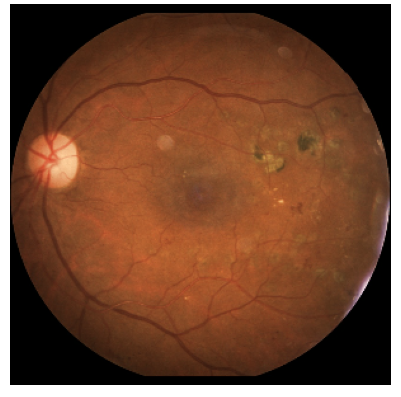
Figure 1 shows an example of the prediction given by a neural network model in order to detect patients suffering from diabetic retinopathy, which is a eye disease caused by diabetes complication [4]. The model was first trained to differentiate healthy patients from diseased ones [6] with images from an open source dataset [5] coming from fundus examinations.
Then, an image, such as the one in Figure 1, which is of a diseased patient, is given to the model which realises a prediction. We notice that the prediction is correct since the probability, estimated by the model, that the image belongs to a diseased patient is very high. However, we would like to know on which parts of the image the model has based to do the prediction. This will allow to find the most important areas in the decision made.
These methods we are going to present belong to the explainability field, often abbreviated as XAI for eXplainable Artificial Intelligence. These methods allow to visualise the most important area in the model’s prediction [7, 8].
99,89% be sick according the model
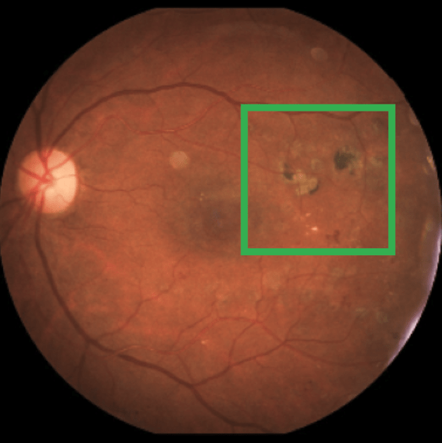
Visualisation of convolutions
Once the neural network has been trained and its coefficients set, a better way to understand the model decision is to look in detail at its different convolutional filters. It is in fact these layers that handle the image the most, particularly by integrating pixels intensity as well as their spatial proximity.
However, a neural network is generally made up of a high number of convolutional filters, at least ten for older models and up to around a hundred for today’s models, preventing them from being all analysed in detail.
Thus, a first approach was published in the article [9] in 2016 taking into account the last convolutional layer of a network. Named Class Activation Map (abbreviated as CAM), this method is based on the outputs, which vary depending on the image used, of this convolutional layer to estimate the important areas of the convolution regarding the image. Given that the size of the last convolutional layer is much smaller than the original image, it is then necessary to resize the CAM result in order to correctly visualise the most important areas in the prediction provided by the model.
Nevertheless, the CAM method has the disadvantage of being based only on a specific architecture (a convolutional layer followed by a Global Average Pooling layer), which prevents its use in many cases. Thus, the method called GradCAM, published in 2017 in the article [10], is based on CAM without any architecture restriction, except for the requirement to keep a convolutional layer. Furthermore GradCAM uses gradients, hence its name, of the layers to estimate the impact of each area.
Moreover, this method allows to understand the impact of convolution layers at different levels of the neural network, and not only on the last one. It is then possible to follow the evolution of the image processing in the model. Figure 3 shows the results provided by the GradCAM++ method, an improvement of GradCAM published in 2018 [11], for three convolutional layers. Results are scaled to the size of the original image and then overlaid on the latter.
Initial convolutional layer
Intermediate convolutional layer
Last convolution layer

The result on the left (initial) is provided by a convolution layer located at the beginning of the neural network. We notice that no area stands out, the image seems to be used as a whole.
The result on the centre (intermediate) comes from a convolution layer located in the middle of the neural network. This time, the convolution seems to focus on a limited area of the image, which is the one identify as an eye lesion, a clear sign of the disease. The last result, on the right (last) is produced by the last convolutional layer. Once again, an area stands out, but it is not the same as the one before.
Thus, Class Activation Map methods give a better insight into the processing of the image in the model, and thus into its decision process. Nevertheless, as noted in Figure 3, the results can be noticeably different depending on the layer of the neural network to which the CAM method is applied. Consequently, it would be interesting to have a more global method, in order to take into account in one visualisation, the impacts of each layer of the neural network.
Saliency Map
Saliency Map methods aim to look at the impact of each pixel on the model prediction, thus providing a general explanation of the decision.
A first version was published in 2013 in the article [12]. This method called Vanilla Gradient calculates the impact of pixels by approximating their respective gradient on the prediction.
This method can be improved by using several slightly perturbed versions of the original image, via the addition of Gaussian noise. These different results are then averaged to form the final visualisation. This improvement, named SmoothGrad and published in 2017 in the paper [13], allows to better consider the different parts of the image. The saliency map produced by the Vanilla Gradient method often focuses only on one area.
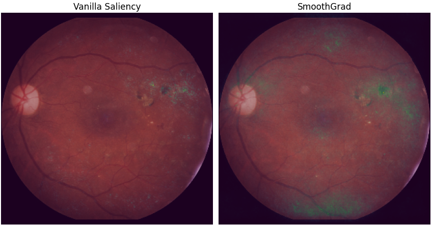
Figure 4 shows the results of the two saliency map methods presented above. The Vanilla Gradient method mainly highlights the area identified a priori as a clinical sign of the disease. While its enhancement using the SmoothGrad algorithm shows three additional areas: one at the top of the image (as was the case for the GradCAM ++ result for the last convolutional layer), an area slightly above the fovea, and the bottom part of the image. Nevertheless, the most prominent and flickering area is always the lesion on the right side of the image, indicating good consistency between the methods.
Although these different visualisation methods allow a better understanding of the model, they remain specific to neural networks. Therefore, it would be interesting to have a method applicable to any type of model.
LIME
Explainability methods that apply to all types of models are called « agnostic ». The Local Interpretable Modelagnostic Explanations method (LIME) is one of them. It was published in 2016 in the paper [14]. It uses image perturbations to identify the areas that impact the prediction the most.
Explainability methods that apply to all types of models are called agnostic
The first step is to segment the image of interest. Figure 5 shows an example of image segmentation. The different areas are called superpixels with the so-called Quickshift method.
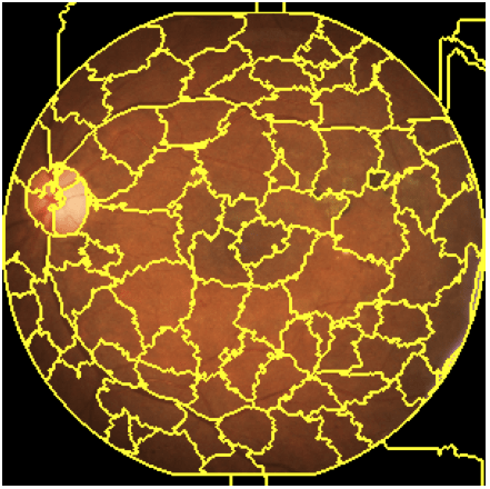
It is important not to segment the image into too many areas as this can lead to long calculation times. Indeed, the LIME method disturbs the image by hiding some areas (one or several areas at the same time) from the segmentation (by filling them with a single colour, black for example). It then studies the prediction associated with each of the peturbations.
Figure 6 shows different perturbations and the respective predictions given by the model. The original image, on the left, is associated with a 99.89% risk of being ill. The middle image shows a disruption of the superpixel containing the occular lesion. The prediction associated with this image is significantly lower than that associated with the original image (72%). For the image on the right, the prediction is almost unchanged (95%). While it shows a disturbance of a larger area than the middle one. This reveals that the central area of the image is not decisive for the prediction.
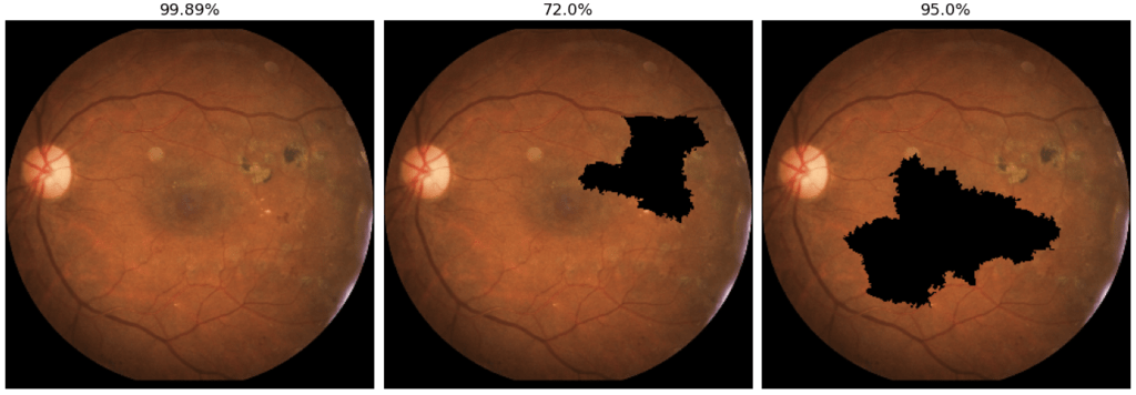
The LIME method repeats this perturbation-prediction process many times, and then weights each perturbation according to its similarity to the original image.
Thus, slighly altered image have higher weight. For example, the middle image in Figure 6 has more weight than the left one, since it has a smaller occluded area than the latter. Finally, the algorithm identifies the most critical areas by searching for the peturbations with the largest deviation from the baseline prediction. In our case, the superpixels on the clinical sign are considered more impactful than the central superpixels, since the deviation from the baseline prediction is larger for this image (72% vs. 99.89%).
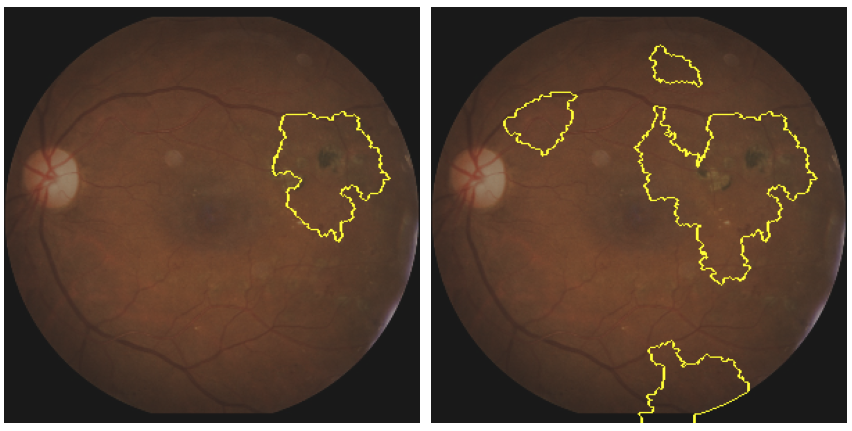
Figure 7 shows the results of the LIME method applied to our case. A threshold can be defined to select the areas (i.e. superpixels) with the highest impact.
By varying this threshold, it is possible to see not only the most decisive area for the prediction (left image), but also the secondary areas that also played a role in the prediction (right image).
Once again, we see that the area that explains most of the prediction is the one containing the microvascular lesion. We also notice that other parts of the image (at the bottom and close to the fovea) help to explain the prediction. The results are similar to those obtained with the saliency map, reflecting a strong consistency between these methods.
Conclusion
The significant improvement in the performance of image analysis models has led to the development of many methods to explain the decisions made by these models. These check that the models used are based on relevant elements such as clinical signs and not on artefacts.
However, these methods have limitations. They are very effective in cases where the clinical signs are in restricted areas. They are less relevant when the model is based on more global patterns. This type of signal is often encountered in medical imaging. For example, diabetic retinopathy is often detected thanks to the density and tortuosity of retinal blood vessels [16]. Current visualisation methods struggle to represent such global signals.
However, these recent advances have improved the quality of predictive imaging models. This has not only increased the reliability of the predictions but also increased the confidence of the experts in the predictions through the identification of clinical signs.
Automatic image analysis has seen its performance grow strongly in recent years. These recent advances improve the construction of predictive

Healthcare journey
Our journey design begins with the first recording of a patient for a reason in a healthcare facility until the
Bibliography
[1] S. K. Zhou, H. Greenspan, C. Davatzikos, J. S. Duncan, B. van Ginneken, A. Madabhushi, J. L.Prince, D. Rueckert, and R. M. Summers, “A review of deep learning in medical imaging : Imagingtraits, technology trends, case studies with progress highlights, and future promises,”Proceedingsof the IEEE, 2021.
[2] J. R. Zech, M. A. Badgeley, M. Liu, A. B. Costa, J. J. Titano, and E. K. Oermann, “Confoundingvariables can degrade generalization performance of radiological deep learning models,”arXivpreprint arXiv :1807.00431, 2018.
[3] S. Lapuschkin, S. Wäldchen, A. Binder, G. Montavon, W. Samek, and K.-R. Müller, “Unmaskingclever hans predictors and assessing what machines really learn,”Nature communications, vol. 10,no. 1, pp. 1–8, 2019.
[4]"Rétinopathiediabétique-snof.”https://www.snof.org/encyclopedie/r%C3%A9tinopathie-diab%C3%A9tique. Accessed : 2020.
[5] “Eye-quality (eyeq) assessment dataset.”https://github.com/HzFu/EyeQ. Accessed : 2019.
[6] H. Fu, B. Wang, J. Shen, S. Cui, Y. Xu, J. Liu, and L. Shao, “Evaluation of retinal image qualityassessment networks in different color-spaces,” inInternational Conference on Medical ImageComputing and Computer-Assisted Intervention, pp. 48–56, Springer, 2019.
[7] M. Poceviči ̄ut ̇e, G. Eilertsen, and C. Lundström, “Survey of xai in digital pathology,” inArtificialIntelligence and Machine Learning for Digital Pathology, pp. 56–88, Springer, 2020.
[8] D. T. Huff, A. J. Weisman, and R. Jeraj, “Interpretation and visualization techniques for deeplearning models in medical imaging,”Physics in Medicine & Biology, vol. 66, no. 4, p. 04TR01,2021.
[9] B. Zhou, A. Khosla, A. Lapedriza, A. Oliva, and A. Torralba, “Learning deep features for dis-criminative localization,” inProceedings of the IEEE conference on computer vision and patternrecognition, pp. 2921–2929, 2016.
[10] R. R. Selvaraju, M. Cogswell, A. Das, R. Vedantam, D. Parikh, and D. Batra, “Grad-cam :Visual explanations from deep networks via gradient-based localization,” inProceedings of theIEEE international conference on computer vision, pp. 618–626, 2017.
[11] A. Chattopadhay, A. Sarkar, P. Howlader, and V. N. Balasubramanian, “Grad-cam++ : Genera-lized gradient-based visual explanations for deep convolutional networks,” in2018 IEEE WinterConference on Applications of Computer Vision (WACV), pp. 839–847, IEEE, 2018.
[12] K. Simonyan, A. Vedaldi, and A. Zisserman, “Deep inside convolutional networks : Visualisingimage classification models and saliency maps,”arXiv preprint arXiv :1312.6034, 2013.
[13] D. Smilkov, N. Thorat, B. Kim, F. Viégas, and M. Wattenberg, “Smoothgrad : removing noiseby adding noise,”arXiv preprint arXiv :1706.03825, 2017.
[14] M. T. Ribeiro, S. Singh, and C. Guestrin, “" why should i trust you ?" explaining the predictions ofany classifier,” inProceedings of the 22nd ACM SIGKDD international conference on knowledgediscovery and data mining, pp. 1135–1144, 2016.
[15] “Comparison of segmentation and superpixel algorithms - scikit-image.”https://scikit-image.org/docs/stable/auto_examples/segmentation/plot_segmentations.html.Accessed :2020.
[16] M. Alam, Y. Zhang, J. I. Lim, R. Chan, M. Yang, and X. Yao, “Quantitative oct angiographyfeatures for objective classification and staging of diabetic retinopathy,”Retina (Philadelphia,Pa.).